Overfitting occurs when a machine learning model learns the training data too well, including noise and random fluctuations, causing it to perform excellently on training data but poorly on new, unseen data. It happens when models are too complex, training data is insufficient, or training continues too long. Prevention techniques include using more data, regularization, cross-validation, early stopping, and simplifying model architecture.
Introduction: The Memorization Problem
Imagine a student preparing for a math exam by memorizing answers to 100 practice problems without understanding the underlying mathematical principles. When the exam presents similar but slightly different problems, the student struggles because they memorized specific solutions rather than learning general problem-solving techniques. This is precisely what happens when machine learning models overfit.
Overfitting is one of the most fundamental and pervasive challenges in machine learning. It’s the reason a model can achieve 99% accuracy during training yet perform no better than random guessing in production. It’s why adding more features sometimes makes models worse. It’s the silent killer of countless machine learning projects that looked promising in development but failed when deployed.
Understanding overfitting is crucial because it represents the gap between performing well on data you’ve seen and performing well on data you haven’t seen—which is the entire point of machine learning. A model that only works on its training data is useless for making real-world predictions. The art and science of machine learning largely revolve around building models that generalize: learning true underlying patterns while ignoring noise and spurious correlations.
This comprehensive guide explores overfitting from every angle. You’ll learn what it is, why it happens, how to detect it early, and most importantly, proven techniques to prevent it. Whether you’re building your first model or optimizing production systems, mastering overfitting prevention is essential for creating reliable, effective machine learning solutions.
What is Overfitting? Understanding the Core Concept
Overfitting occurs when a model learns patterns specific to the training data—including noise, outliers, and random fluctuations—rather than learning the underlying true patterns that generalize to new data.
The Essence of Overfitting
Think of overfitting as the difference between:
Understanding (good generalization):
- Learning that houses with more square footage tend to cost more
- Understanding that customers who engage frequently are less likely to churn
- Recognizing that emails with certain word patterns are likely spam
Memorization (overfitting):
- Learning that house #42 at 123 Main St sold for exactly $325,000
- Memorizing that customer ID 7821 purchased on Thursdays
- Remembering that email #523 was spam because it contained “meeting” and “tomorrow”
The memorization approach achieves perfect accuracy on training data but provides no useful ability to predict new cases.
Visual Understanding: The Curve Fitting Example
Consider fitting a curve to predict house prices based on square footage:
Appropriate Fit (good generalization):
- Smooth curve capturing general trend
- Prices increase with square footage
- Allows for natural variation
- Works well for new houses
Overfit (memorization):
- Wiggly curve passing through every training point exactly
- Captures every random fluctuation and outlier
- Perfect on training data (zero error)
- Terrible on new data (large errors)
The overfit model is more complex, fits training data better, but generalizes worse—the hallmark of overfitting.
The Performance Gap
Overfitting manifests as a gap between training and validation/test performance:
Well-Generalized Model:
- Training accuracy: 85%
- Validation accuracy: 83%
- Test accuracy: 84%
- Small gap indicates good generalization
Overfit Model:
- Training accuracy: 99%
- Validation accuracy: 72%
- Test accuracy: 70%
- Large gap indicates severe overfitting
The overfit model appears superior based on training data but is actually far worse at the task that matters: predicting new examples.
Overfitting in Different Contexts
Overfitting appears differently across machine learning tasks:
Classification:
- Model learns specific training examples rather than decision boundaries
- Achieves near-perfect training accuracy
- Misclassifies many new examples
- Example: Spam filter that works perfectly on training emails but fails on new spam tactics
Regression:
- Model fits training points exactly, including noise
- Zero or near-zero training error
- Large errors on new predictions
- Example: Stock price predictor that perfectly “predicts” historical prices but fails on future prices
Clustering:
- Creates too many small clusters capturing noise
- Each cluster fits training idiosyncrasies
- Doesn’t reveal meaningful groupings
- Example: Customer segmentation that creates 100 micro-segments instead of 5 meaningful ones
Neural Networks:
- Network memorizes training examples in its many parameters
- Can achieve 100% training accuracy
- Representations don’t transfer to new data
- Example: Image classifier that memorizes training images pixel-by-pixel
Why Does Overfitting Happen? Root Causes
Understanding why overfitting occurs helps prevent it. Several factors contribute:
Cause 1: Model Complexity
Models with many parameters relative to available data can fit training data perfectly, including noise.
Example: Polynomial Regression
Predicting house prices from square footage:
Simple model (linear: y = mx + b):
- 2 parameters (m and b)
- Can’t fit every training point exactly
- Captures general trend
- Generalizes well
Complex model (degree-10 polynomial):
- 11 parameters
- Can fit training points exactly
- Captures noise as if it’s signal
- Generalizes poorly
Principle: With enough parameters, you can fit any finite dataset perfectly, learning nothing useful about underlying patterns.
Real-World Examples:
- Deep neural network with millions of parameters trained on thousands of examples
- Decision tree allowed to grow until each leaf contains one example
- Feature set with thousands of features for hundreds of examples
Cause 2: Insufficient Training Data
Small datasets don’t provide enough information to distinguish true patterns from noise.
Analogy: Imagine learning about a country’s weather by visiting for one week. You might conclude it rains every Wednesday if it happened to rain the two Wednesdays you were there. With data from 52 weeks, you’d learn the actual weather patterns.
Example:
- Problem: Predict customer churn (complex behavior influenced by many factors)
- Data: 100 customers (50 churned, 50 retained)
- Risk: With limited data, model might learn spurious correlations—”customers whose names start with ‘A’ churn more”—that happened by chance
Rule of Thumb: You generally need at least 10-20 examples per feature, though this varies widely by problem.
Cause 3: Training Too Long
Models can initially learn genuine patterns, then progressively overfit as training continues.
Training Progression:
Early epochs (iterations):
- Model learns general patterns
- Training and validation errors both decrease
- Good generalization
Optimal point:
- Validation error reaches minimum
- Best generalization achieved
- Ideal stopping point
Later epochs:
- Training error continues decreasing
- Validation error starts increasing
- Model learning training-specific noise
- Overfitting occurs
This phenomenon is especially common in neural networks trained with gradient descent.
Cause 4: Noise in Data
Real-world data contains noise: measurement errors, mislabeled examples, random variations, outliers.
Example Issues:
- Medical images mislabeled by human reviewers
- Sensor data with measurement errors
- User behavior influenced by random factors
- Data entry mistakes
Problem: Models try to fit everything in training data, treating noise as if it’s meaningful signal. The model “explains” random fluctuations that don’t reflect true underlying patterns.
Cause 5: Too Many Features
High-dimensional feature spaces (many features) make overfitting more likely, especially with limited data.
Curse of Dimensionality:
- In high dimensions, data points become sparse
- Models can find spurious patterns in sparse regions
- Overfitting risk increases dramatically
Example:
- 10,000 features (genes, pixels, word counts)
- 500 training examples
- Model finds features that correlate with labels by chance
- These correlations don’t hold on new data
Cause 6: Inappropriate Model Choice
Using unnecessarily complex models for simple problems invites overfitting.
Example:
- Problem: Predict whether temperature is above/below 60°F based on month
- Appropriate: Simple threshold or linear model
- Overkill: Deep neural network with 10 layers
- Result: Network overfits, learning training set idiosyncrasies
Principle: Model complexity should match problem complexity. Simple problems need simple models.
How to Detect Overfitting: Warning Signs
Recognizing overfitting early allows you to address it before deployment.
Sign 1: Large Training-Validation Gap
Clear Indicator: Training performance significantly exceeds validation/test performance
Example:
Training accuracy: 95%
Validation accuracy: 68%
Gap: 27 percentage points → Strong overfittingWhat to Look For:
- Small gap (2-5%): Normal, acceptable
- Medium gap (5-15%): Some overfitting, room for improvement
- Large gap (>15%): Severe overfitting, needs addressing
Sign 2: Near-Perfect Training Performance
Warning: 99-100% training accuracy or near-zero training loss
Why Suspicious: Real-world data has noise. Perfect fitting suggests memorization.
Exception: Very simple problems with clean data might legitimately achieve near-perfect training accuracy.
Example:
Problem: Detect fraudulent transactions (complex, noisy)
Training accuracy: 99.9%
→ Likely overfitting; problem is too complex for such perfectionSign 3: Performance Degradation Over Training Time
Pattern:
- Validation loss decreases initially
- Then starts increasing while training loss continues decreasing
Interpretation: Model started generalizing well but is now memorizing training data
Visual Pattern:
Training Loss:     \  \   \    \     (continuously decreasing)
Validation Loss:    \  \   \    /      / (decreases then increases)
                            ↑
                      Overfitting begins
Sign 4: Unstable Model Predictions
Symptom: Small changes in training data cause large changes in model
Test:
- Train model on 95% of training data
- Train again on different 95%
- Compare predictions
Overfit Models: Drastically different predictions Well-Generalized Models: Similar predictions
Sign 5: Poor Performance on New Data
Ultimate Test: Deploy model and monitor real-world performance
Overfitting Pattern:
- Development accuracy: 90%
- Production accuracy: 65%
- Performance drops significantly with real data
Sign 6: Unusual Feature Importance
Warning Sign: Model heavily relies on features that shouldn’t matter based on domain knowledge
Example:
Problem: Predict loan default
Top feature: Customer ID
→ Red flag! Customer ID shouldn't predict default
→ Model likely memorizing training examplesLegitimate features should make intuitive sense given the problem.
Sign 7: Complex Decision Boundaries
Visual Inspection: For 2D problems, plot decision boundaries
Overfit Pattern:
- Extremely wiggly, convoluted boundaries
- Boundaries wrap around individual points
- Fits training points exactly but illogically
Well-Generalized:
- Smooth, reasonable boundaries
- Captures general patterns
- Some training points may be on wrong side (acceptable)
How to Prevent Overfitting: Proven Techniques
Preventing overfitting requires a multi-faceted approach. Different techniques work better for different scenarios.
Technique 1: Get More Training Data
Most Effective Solution: More data reduces overfitting dramatically
Why It Works:
- Harder to memorize larger datasets
- More data reveals true patterns vs. noise
- Spurious correlations don’t repeat across more examples
- Model learns generalizable patterns
How Much More?:
- Rule of thumb: 10-20x more samples than features
- Deep learning: Often needs 1000s to millions of examples
- Simple models: Can work with hundreds of examples
Obtaining More Data:
Data Collection:
- Gather additional labeled examples
- Extend data collection period
- Expand to new sources
Data Augmentation:
- Images: Rotate, flip, crop, adjust brightness/contrast
- Text: Synonym replacement, back-translation
- Audio: Add noise, change speed, pitch shift
- Time series: Jittering, scaling, window slicing
Synthetic Data:
- Generate artificial examples
- Use domain knowledge to create realistic variations
- GANs (Generative Adversarial Networks) for complex data
Example:
Original dataset: 1,000 images
After augmentation: 10,000 images (10x per original)
Result: Model generalizes much betterTechnique 2: Regularization
Principle: Add penalty for model complexity during training
How It Works: Cost function becomes:
Total Loss = Prediction Error + Complexity PenaltyModel must balance fitting data well vs. staying simple.
L2 Regularization (Ridge)
Penalty: Sum of squared parameter values
Effect:
- Shrinks parameter values toward zero
- Prefers many small weights over few large weights
- Smooth decision boundaries
Implementation:
from sklearn.linear_model import Ridge
model = Ridge(alpha=1.0) # alpha controls strengthWhen to Use: Default choice for regularization
L1 Regularization (Lasso)
Penalty: Sum of absolute parameter values
Effect:
- Drives some parameters to exactly zero
- Performs automatic feature selection
- Creates sparse models
Implementation:
from sklearn.linear_model import Lasso
model = Lasso(alpha=0.1)When to Use: When you want feature selection or sparse models
Elastic Net
Combination: Mix of L1 and L2
Benefits:
- Gets advantages of both
- More stable than pure L1
- Still provides some feature selection
Dropout (Neural Networks)
Method: Randomly deactivate neurons during training
Process:
- Each training step, randomly set 20-50% of neurons to zero
- Forces network not to rely on specific neurons
- Creates ensemble effect
Implementation:
model.add(Dense(128, activation='relu'))
model.add(Dropout(0.5)) # Drop 50% of neuronsWhy It Works:
- Prevents co-adaptation of neurons
- Makes network robust to missing information
- Reduces overfitting significantly
Technique 3: Cross-Validation
Method: Evaluate model on multiple different data splits
Process:
- Divide data into K folds
- Train K times, each time using different fold for validation
- Average performance across all folds
Benefits:
- More robust performance estimate
- Detects if model is overfitting to specific validation split
- Makes better use of limited data
Implementation:
from sklearn.model_selection import cross_val_score
scores = cross_val_score(model, X, y, cv=5)
print(f"Average accuracy: {scores.mean():.3f} (+/- {scores.std():.3f})")Recommendation: Use 5-fold or 10-fold cross-validation
Technique 4: Early Stopping
Method: Stop training when validation performance stops improving
Process:
- Monitor validation loss during training
- When validation loss stops decreasing (or starts increasing)
- Stop training
- Optionally restore model to best validation performance
Why It Works: Catches model at the point where it’s learned patterns but not yet memorized training data
Implementation:
from keras.callbacks import EarlyStopping

early_stop = EarlyStopping(
    monitor='val_loss',
    patience=10,  # Wait 10 epochs for improvement
    restore_best_weights=True
)

model.fit(X_train, y_train,
          validation_data=(X_val, y_val),
callbacks=[early_stop])Parameters:
- Patience: How many epochs to wait before stopping
- Restore best: Use weights from best epoch, not final epoch
Technique 5: Simplify Model Architecture
Principle: Use the simplest model that works adequately
Approaches:
Reduce Model Capacity:
- Fewer layers in neural networks
- Smaller trees in decision tree models
- Fewer parameters overall
Example – Neural Network:
# Complex (prone to overfitting)
model = Sequential([
    Dense(512, activation='relu'),
    Dense(512, activation='relu'),
    Dense(256, activation='relu'),
    Dense(256, activation='relu'),
    Dense(10, activation='softmax')
])

# Simpler (better generalization)
model = Sequential([
    Dense(128, activation='relu'),
    Dense(64, activation='relu'),
    Dense(10, activation='softmax')
])Decision Trees:
- Limit maximum depth
- Require minimum samples per leaf
- Limit maximum number of leaves
Start Simple: Begin with simple models, add complexity only if needed
Technique 6: Feature Selection
Goal: Remove irrelevant or redundant features
Why It Helps:
- Fewer features = fewer opportunities for spurious correlations
- Reduces curse of dimensionality
- Simpler models less prone to overfitting
Methods:
Filter Methods (before modeling):
- Correlation analysis
- Statistical tests
- Mutual information
- Remove low-variance features
Wrapper Methods (using model performance):
- Recursive feature elimination
- Forward/backward selection
Embedded Methods (built into training):
- L1 regularization (Lasso)
- Tree-based feature importance
Example:
from sklearn.feature_selection import SelectKBest, f_classif

# Select top 20 features
selector = SelectKBest(f_classif, k=20)
X_selected = selector.fit_transform(X_train, y_train)Technique 7: Ensemble Methods
Principle: Combine multiple models to reduce overfitting
Why It Works:
- Individual models might overfit differently
- Averaging reduces impact of overfitting in any single model
- Ensemble generalizes better than components
Common Approaches:
Bagging (Bootstrap Aggregating):
- Train multiple models on different data subsets
- Average predictions
- Example: Random Forests
Boosting:
- Train models sequentially, each correcting previous errors
- Example: XGBoost, AdaBoost
Stacking:
- Train multiple diverse models
- Train meta-model on their predictions
Example:
from sklearn.ensemble import RandomForestClassifier

# Random Forest is ensemble of decision trees
rf = RandomForestClassifier(n_estimators=100)
rf.fit(X_train, y_train)
# Less overfitting than single decision treeTechnique 8: Data Preprocessing and Normalization
Standardization:
from sklearn.preprocessing import StandardScaler

scaler = StandardScaler()
X_train_scaled = scaler.fit_transform(X_train)
X_val_scaled = scaler.transform(X_val) # Use training statisticsWhy It Helps:
- Makes optimization more stable
- Prevents features with large scales from dominating
- Helps regularization work effectively
Important: Fit scaler only on training data, apply to validation/test
Technique 9: Noise Injection
Method: Add random noise during training
Types:
Input Noise: Add small random perturbations to input features Weight Noise: Add noise to model parameters during training Label Smoothing: For classification, use soft labels (0.9, 0.1) instead of hard labels (1.0, 0.0)
Why It Works: Forces model to be robust to small variations, preventing memorization
Technique 10: Batch Normalization
Method: Normalize inputs to each layer during training
Benefits:
- Stabilizes training
- Allows higher learning rates
- Has regularization effect
- Reduces internal covariate shift
Implementation:
model.add(Dense(128))
model.add(BatchNormalization())  # Add after dense layer
model.add(Activation('relu'))Practical Example: Preventing Overfitting in Image Classification
Let’s walk through a complete example addressing overfitting.
Initial Problem
Task: Classify images of cats vs. dogs Training Data: 2,000 images (1,000 per class) Validation Data: 500 images
Attempt 1: Initial Model (Overfits)
model = Sequential([
    Conv2D(64, (3, 3), activation='relu'),
    MaxPooling2D((2, 2)),
    Conv2D(128, (3, 3), activation='relu'),
    MaxPooling2D((2, 2)),
    Conv2D(256, (3, 3), activation='relu'),
    MaxPooling2D((2, 2)),
    Flatten(),
    Dense(512, activation='relu'),
    Dense(512, activation='relu'),
    Dense(1, activation='sigmoid')
])

# Train for 50 epochsResults:
- Training accuracy: 98%
- Validation accuracy: 72%
- Diagnosis: Severe overfitting (26% gap)
Attempt 2: Add Dropout
model = Sequential([
    Conv2D(64, (3, 3), activation='relu'),
    MaxPooling2D((2, 2)),
    Dropout(0.25),  # Add dropout
    Conv2D(128, (3, 3), activation='relu'),
    MaxPooling2D((2, 2)),
    Dropout(0.25),  # Add dropout
    Conv2D(256, (3, 3), activation='relu'),
    MaxPooling2D((2, 2)),
    Dropout(0.25),  # Add dropout
    Flatten(),
    Dense(512, activation='relu'),
    Dropout(0.5),  # Higher dropout in dense layers
    Dense(512, activation='relu'),
    Dropout(0.5),
    Dense(1, activation='sigmoid')
])Results:
- Training accuracy: 89%
- Validation accuracy: 79%
- Improvement: Gap reduced to 10%
Attempt 3: Add Data Augmentation
from tensorflow.keras.preprocessing.image import ImageDataGenerator

datagen = ImageDataGenerator(
    rotation_range=20,
    width_shift_range=0.2,
    height_shift_range=0.2,
    horizontal_flip=True,
    zoom_range=0.2
)

# Train with augmented data
model.fit(datagen.flow(X_train, y_train, batch_size=32),
          validation_data=(X_val, y_val),
epochs=50)Results:
- Training accuracy: 86%
- Validation accuracy: 82%
- Improvement: Gap reduced to 4%
Attempt 4: Simplify Architecture + Early Stopping
# Simpler model
model = Sequential([
    Conv2D(32, (3, 3), activation='relu'),  # Fewer filters
    MaxPooling2D((2, 2)),
    Dropout(0.25),
    Conv2D(64, (3, 3), activation='relu'),  # Fewer filters
    MaxPooling2D((2, 2)),
    Dropout(0.25),
    Flatten(),
    Dense(128, activation='relu'),  # Smaller dense layer
    Dropout(0.5),
    Dense(1, activation='sigmoid')
])

# Add early stopping
early_stop = EarlyStopping(
    monitor='val_loss',
    patience=5,
    restore_best_weights=True
)

model.fit(datagen.flow(X_train, y_train, batch_size=32),
          validation_data=(X_val, y_val),
          epochs=100,  # Allow many epochs
callbacks=[early_stop]) # But stop earlyResults:
- Training accuracy: 84%
- Validation accuracy: 83%
- Final State: Minimal gap, good generalization
Lessons Learned
Progressive Improvement:
- Start with overfitting model
- Add dropout → 7% improvement
- Add data augmentation → 3% more improvement
- Simplify + early stopping → Final 1% improvement
Final Model Characteristics:
- Simpler architecture (fewer parameters)
- Dropout for regularization
- Data augmentation (effective 10x more data)
- Early stopping (stopped at epoch 23, not 100)
- Good balance: learns patterns without memorizing
Domain-Specific Overfitting Challenges
Different domains face unique overfitting challenges:
Computer Vision
Challenges:
- High-dimensional input (thousands of pixels)
- Need large datasets
- Easy to memorize specific images
Solutions:
- Data augmentation (rotation, flipping, cropping)
- Transfer learning (pre-trained models)
- Dropout and batch normalization
- Progressive resizing
Natural Language Processing
Challenges:
- High-dimensional sparse features
- Variable-length inputs
- Domain-specific vocabulary
Solutions:
- Word embeddings reduce dimensionality
- Dropout in recurrent layers
- Attention mechanisms with dropout
- Data augmentation (back-translation, synonym replacement)
Time Series
Challenges:
- Temporal dependencies
- Limited data often available
- Easy to overfit to recent patterns
Solutions:
- Strictly temporal validation splits
- Regularization
- Simpler models (ARIMA before deep learning)
- Ensemble methods
Tabular Data
Challenges:
- Often limited samples
- Mixed feature types
- Many irrelevant features possible
Solutions:
- Feature selection crucial
- Tree-based models naturally regularize
- Cross-validation
- Feature engineering with domain knowledge
Monitoring for Overfitting in Production
Detecting overfitting doesn’t end at deployment:
Continuous Monitoring
Track Performance:
- Monitor prediction accuracy on new data
- Compare to expected performance from validation
- Alert if performance drops significantly
Example:
Expected accuracy (from validation): 85%
Week 1 production: 84% → Normal variation
Week 2 production: 83% → Still acceptable
Week 3 production: 76% → Alert! InvestigateConcept Drift
Challenge: World changes, patterns shift over time
Symptoms:
- Model performance degrades gradually
- Feature distributions change
- Relationship between features and labels evolves
Solutions:
- Regular retraining with fresh data
- Online learning algorithms
- Adaptive models
- Monitor feature distributions
A/B Testing
Method: Compare new models against production model
Process:
- Deploy new model to small percentage of traffic
- Compare performance to existing model
- Gradually increase if better, rollback if worse
Prevents: Deploying overfit models that looked good in development
Best Practices Summary
During Development
- Always use separate validation/test sets
- Start simple, add complexity only if needed
- Monitor training vs. validation performance
- Use cross-validation for robust estimates
- Apply regularization by default
- Implement early stopping
- Visualize learning curves
Model Selection
- Prefer simpler models when performance is similar
- Use ensemble methods for better generalization
- Select features carefully
- Match model complexity to data size
Data Strategy
- Collect more data when possible
- Use data augmentation creatively
- Clean data to reduce noise
- Ensure validation set is representative
Production
- Monitor performance continuously
- Compare to validation estimates
- Retrain regularly with new data
- Use A/B testing for new models
- Have rollback plans
Comparison: Overfitting Prevention Techniques
| Technique | Effectiveness | Computational Cost | Ease of Implementation | Best For |
|---|---|---|---|---|
| More Data | Very High | Low (but data collection costly) | Easy | All scenarios |
| Data Augmentation | High | Low | Easy | Images, text, audio |
| Regularization (L1/L2) | High | Very Low | Very Easy | Linear models, simple NNs |
| Dropout | Very High | Low | Easy | Neural networks |
| Early Stopping | High | Low | Easy | Iterative training |
| Cross-Validation | Medium (detection) | High | Medium | Model selection |
| Simpler Model | High | Low | Easy | When complex model unnecessary |
| Feature Selection | Medium-High | Medium | Medium | High-dimensional data |
| Ensemble Methods | High | High | Medium | Most scenarios |
| Batch Normalization | Medium | Low | Easy | Deep neural networks |
Conclusion: Balancing Complexity and Generalization
Overfitting represents one of machine learning’s central challenges: the tension between learning from data and generalizing beyond it. Models must be complex enough to capture true patterns but simple enough not to memorize noise. Too simple and they underfit, missing important relationships. Too complex and they overfit, learning spurious correlations.
Understanding overfitting means recognizing that training performance alone tells you nothing about model quality. A model with 100% training accuracy might be useless if it achieves only 60% on new data. The gap between training and validation performance is often more informative than the absolute numbers.
Preventing overfitting requires a multi-faceted approach:
More data is the most powerful solution when available, diluting noise and revealing true patterns.
Regularization constrains model complexity, forcing simpler explanations that generalize better.
Cross-validation provides robust performance estimates, detecting overfitting early.
Early stopping catches models at the sweet spot before memorization begins.
Simpler architectures reduce overfitting risk by limiting model capacity.
Feature selection removes opportunities for spurious correlations.
Ensemble methods average out individual model biases and overfitting.
The key is recognizing that no single technique solves overfitting completely. Successful practitioners combine multiple approaches: collecting sufficient data, engineering relevant features, choosing appropriate model complexity, applying regularization, validating rigorously, and monitoring production performance.
Overfitting isn’t a bug to be eliminated but a fundamental tradeoff to be managed. Some overfitting is acceptable—a small gap between training and validation performance is normal. The goal isn’t zero overfitting but rather finding the right balance where models capture genuine patterns while maintaining the ability to generalize.
As you build machine learning systems, make overfitting prevention a core part of your workflow, not an afterthought. Monitor the training-validation gap continuously. Start simple and add complexity only when justified. Use regularization by default. Validate rigorously. The time invested in preventing overfitting pays dividends when models actually work in production, delivering value rather than disappointing with performance that doesn’t match development estimates.
Master overfitting prevention, and you’ve mastered one of machine learning’s most critical skills—building models that don’t just memorize examples but truly learn to solve problems.