The Foundation of Predictive Analytics
Linear regression is one of the simplest yet most powerful tools in the field of statistics and machine learning. It is a method used to model the relationship between a dependent variable and one or more independent variables. By fitting a linear equation to observed data, linear regression can make predictions, establish relationships, and provide insights into data trends. This guide aims to demystify linear regression for beginners, breaking down its concepts, applications, and implementation step-by-step.
Understanding Linear Regression
What is Linear Regression?
Linear regression is a predictive analysis technique used to understand the relationship between variables. The core idea is to fit a line through a scatter plot of data points that best predicts the dependent variable based on the independent variable(s). The simplest form, simple linear regression, involves one independent variable and one dependent variable:
y=β0+β1x+ϵ
Here:
- y is the dependent variable (the outcome we are trying to predict),
- x is the independent variable (the predictor),
- β0 is the intercept (the value of y when x is 0),
- β1 is the slope (the change in y for a one-unit change in x),
- ϵ is the error term (the difference between the observed and predicted values).
Types of Linear Regression
Simple Linear Regression: Involves a single independent variable. It is used to predict the value of a dependent variable based on one independent variable.
Multiple Linear Regression: Involves two or more independent variables. It is used to predict the value of a dependent variable based on multiple independent variables, providing a more comprehensive model.
Key Concepts in Linear Regression
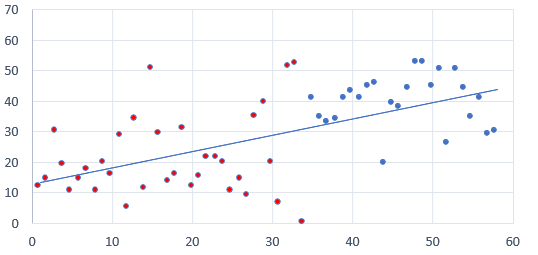
The Line of Best Fit
The line of best fit (or regression line) is the straight line that best represents the data on a scatter plot. The method of least squares is commonly used to determine this line, minimizing the sum of the squares of the vertical distances of the points from the line.
Coefficients
The coefficients (β values) in a linear regression model represent the weight or importance of each independent variable. In simple linear regression, there are two coefficients: the intercept (β0) and the slope (β1).
R-Squared Value
The R-squared value (R²) measures the proportion of the variance in the dependent variable that is predictable from the independent variable(s). It ranges from 0 to 1, with higher values indicating a better fit of the model.
Assumptions of Linear Regression
For linear regression to produce reliable results, certain assumptions must be met:
Linearity: The relationship between the independent and dependent variables should be linear.
Independence: Observations should be independent of each other.
Homoscedasticity: The residuals (differences between observed and predicted values) should have constant variance.
Normality: The residuals should be approximately normally distributed.
Understanding these assumptions is crucial for validating the results of a linear regression model. Violating these assumptions can lead to biased or inaccurate predictions.
Applications of Linear Regression
Linear regression is widely used in various fields due to its simplicity and interpretability. Common applications include:
Economics: Modeling economic indicators, predicting stock prices.
Healthcare: Predicting patient outcomes, analyzing treatment effects.
Marketing: Understanding the relationship between advertising spend and sales, predicting customer behavior.
Environmental Science: Modeling climate change effects, predicting pollution levels.
In the next section, we will delve into the practical implementation of linear regression using Python, covering data preparation, model building, and evaluation techniques. This hands-on approach will help solidify your understanding and enable you to apply linear regression to real-world data.
Practical Implementation of Linear Regression
Data Preparation
Before building a linear regression model, it is crucial to prepare your data properly. This involves gathering, cleaning, and transforming the data to ensure it is suitable for analysis.
Step 1: Importing Libraries
First, you need to import the necessary Python libraries. We’ll use pandas for data manipulation, NumPy for numerical operations, and Scikit-learn for building and evaluating the model.
import pandas as pd
import numpy as np
from sklearn.model_selection import train_test_split
from sklearn.linear_model import LinearRegression
from sklearn.metrics import mean_squared_error, r2_score
import matplotlib.pyplot as plt
Step 2: Loading the Dataset
Load your dataset into a pandas DataFrame. For this example, let’s assume we are using a dataset that contains information about house prices.
# Load dataset
data = pd.read_csv('house_prices.csv')

# Display first few rows of the dataset
print(data.head())
Step 3: Exploring and Cleaning Data
Explore the dataset to understand its structure and check for any missing or inconsistent data. Cleaning the data might involve handling missing values, removing duplicates, and converting data types.
# Check for missing values
print(data.isnull().sum())

# Fill or drop missing values if necessary
data = data.dropna()

# Check data types
print(data.dtypes)
Building the Linear Regression Model
With the data prepared, we can now build our linear regression model.
Step 4: Selecting Features and Target Variable
Choose the independent variables (features) and the dependent variable (target) for the model. In this example, let’s predict house prices based on features like square footage and number of bedrooms.
# Select features and target variable
X = data[['square_footage', 'num_bedrooms']]
y = data['price']
Step 5: Splitting the Data
Split the data into training and testing sets to evaluate the model’s performance on unseen data.
# Split the data into training and testing sets
X_train, X_test, y_train, y_test = train_test_split(X, y, test_size=0.2, random_state=42)
Step 6: Training the Model
Create an instance of the LinearRegression class and fit it to the training data.
# Create and train the model
model = LinearRegression()
model.fit(X_train, y_train)
Step 7: Making Predictions
Use the trained model to make predictions on the testing set.
# Make predictions
y_pred = model.predict(X_test)
Evaluating the Model
Evaluating the performance of the linear regression model is crucial to ensure its accuracy and reliability.
Step 8: Calculating Metrics
Calculate evaluation metrics such as Mean Squared Error (MSE) and R-squared (R²) to assess the model’s performance.
# Calculate MSE and R-squared
mse = mean_squared_error(y_test, y_pred)
r2 = r2_score(y_test, y_pred)

print(f'Mean Squared Error: {mse}')
print(f'R-squared: {r2}')
Step 9: Visualizing the Results
Visualize the predicted values against the actual values to understand the model’s accuracy better.
# Plot predicted vs actual values
plt.scatter(y_test, y_pred, color='blue')
plt.plot([y_test.min(), y_test.max()], [y_test.min(), y_test.max()], 'k--', lw=3)
plt.xlabel('Actual')
plt.ylabel('Predicted')
plt.title('Actual vs Predicted Prices')
plt.show()
This hands-on implementation illustrates the practical steps involved in building, training, and evaluating a linear regression model using Python. By following these steps, you can apply linear regression to your own datasets and gain valuable insights from your data.
In the next section, we will explore more advanced topics related to linear regression, such as handling multicollinearity, regularization techniques, and interpreting the model coefficients to derive meaningful conclusions.
Advanced Topics in Linear Regression
Handling Multicollinearity
Multicollinearity occurs when two or more independent variables in a regression model are highly correlated, leading to unreliable estimates of the model coefficients. This can be detected using Variance Inflation Factor (VIF), which quantifies how much the variance of a regression coefficient is inflated due to multicollinearity.
Detecting Multicollinearity
To detect multicollinearity, calculate the VIF for each independent variable. A VIF value greater than 10 indicates high multicollinearity.
from statsmodels.stats.outliers_influence import variance_inflation_factor

# Calculate VIF for each feature
X_train_with_constant = sm.add_constant(X_train)  # Add a constant term to the model
vif = pd.DataFrame()
vif["Variable"] = X_train_with_constant.columns
vif["VIF"] = [variance_inflation_factor(X_train_with_constant.values, i) for i in range(X_train_with_constant.shape[1])]

print(vif)
Addressing Multicollinearity
If multicollinearity is detected, consider the following approaches to address it:
Remove highly correlated predictors: Drop one of the correlated variables.
Principal Component Analysis (PCA): Transform the predictors into a set of uncorrelated components.
Regularization Techniques: Use techniques like Ridge or Lasso regression, which we will discuss next.
Regularization Techniques
Regularization techniques are used to prevent overfitting by adding a penalty term to the linear regression cost function. Two popular regularization methods are Ridge regression and Lasso regression.
Ridge Regression
Ridge regression adds a penalty term equal to the square of the magnitude of the coefficients. This shrinks the coefficients, reducing their variance and mitigating multicollinearity.
from sklearn.linear_model import Ridge

# Create and train the Ridge regression model
ridge_model = Ridge(alpha=1.0)
ridge_model.fit(X_train, y_train)

# Make predictions and evaluate the model
ridge_pred = ridge_model.predict(X_test)
ridge_mse = mean_squared_error(y_test, ridge_pred)
ridge_r2 = r2_score(y_test, ridge_pred)

print(f'Ridge Regression Mean Squared Error: {ridge_mse}')
print(f'Ridge Regression R-squared: {ridge_r2}')
Lasso Regression
Lasso regression adds a penalty term equal to the absolute value of the magnitude of the coefficients, which can shrink some coefficients to zero. This is useful for feature selection.
from sklearn.linear_model import Lasso

# Create and train the Lasso regression model
lasso_model = Lasso(alpha=0.1)
lasso_model.fit(X_train, y_train)

# Make predictions and evaluate the model
lasso_pred = lasso_model.predict(X_test)
lasso_mse = mean_squared_error(y_test, lasso_pred)
lasso_r2 = r2_score(y_test, lasso_pred)

print(f'Lasso Regression Mean Squared Error: {lasso_mse}')
print(f'Lasso Regression R-squared: {lasso_r2}')
Interpreting Model Coefficients
Interpreting the coefficients of a linear regression model helps in understanding the impact of each predictor on the dependent variable.
Coefficient Interpretation
Intercept (β0\beta_0β0): The expected value of yyy when all predictors are zero.
Slope (β1,β2,…\beta_1, \beta_2, \dotsβ1,β2,…): The change in yyy for a one-unit change in the corresponding predictor, holding other variables constant.
Statistical Significance
Use hypothesis testing to determine the statistical significance of each coefficient. This is often done using p-values, with a common threshold for significance being 0.05.
import statsmodels.api as sm

# Fit the model using statsmodels to get detailed statistics
X_train_with_constant = sm.add_constant(X_train)
sm_model = sm.OLS(y_train, X_train_with_constant).fit()

# Print the summary of the model
print(sm_model.summary())
Linear regression is a foundational technique in statistics and machine learning, providing a straightforward method for predictive modeling and data analysis. By understanding its principles, assumptions, and advanced topics like multicollinearity and regularization, you can build robust and interpretable models. Whether you are predicting economic trends, healthcare outcomes, or marketing success, linear regression offers a powerful tool for making data-driven decisions.